How to simulate a parachute-jumper?
During a computer simulation class we had the task to simulate the physics of a parachute jumper jumping from a plane at a height of 3000 meters. At first we set up the differential equtations for the problem. Two diffential equations apply during the jump. At first the jumper is in a free fall, until the parachute opens and dramaticly decreases the velocity of the jumper. Otherwise the jumper would hit the ground very fast. When the parachute is opened the aerodynamic drag increases and the second differential equtation applies to the simulation. During landing, the jumper absorbs the impact with his legs. A spring constant is assumed for this purpose. This process naturally stops the parachute jump when the ground is touched. This constraint applies to the model at a heigt of 1,2 meter. The model was polished with a PID-Contoller that decays the movement while landing. In the simulation model both ways are present, but the here shown example runs with the PID-controller.
The link of the model works great on mobile or with MS Edge or Chrome on Desktop. Firefox has an issue with it.
Matlab file and the simulation model
The simulation was developed with the program Matlab Simulink. Simulink is a highly sophisticated software from the company MathWorks. With the 1001 features included in Simulink, i was able to create a webview file of the simulation model. To access the webview model please use the link below. I also attach the parameter file of the simulation thats running in Matlab during the simulation.The link of the model works great on mobile or with MS Edge or Chrome on Desktop. Firefox has an issue with it.
>>CLICK HERE FOR THE WEBVIEW OF THE SIMULATION MODEL<<
% Flash 22.04.22
%developed during a lecture / computer simulation of mechtronic systems
%evolved example from the book "Helmut Scherf- Modellbildung und %Simulation"
% Parameter Parachute Jumper
h_0 = 3000 ; % m height of the jump from plane
h_1 = 1500 ; % m height for open the parachute
h_test = 10 ;
h_SP = 1.2 ; % height of legs of the jumper touching the grond
A_S = 0.5 ; % m^2 bodysurface of the jumper
A_FS = 30 ; % m^2 surface ot the opened parachute
m_S = 85 ; % kg mass of the jumper
c_w_F = 1.3 ; % coefficient of drag of the air
rho = 1.2 ; % kg/m^3 air density assumed constant
g = 9.81 ; % m/s^2 gravity
SimTime = 300; %simulation time
k_O = 1/2*c_w_F*rho*A_FS %decay factor with opened parachute
k_L = 1/2*c_w_F*rho*A_S %decay factor of the jumper falling
k_F = 2*g*m_S/0.5; %jumper can carry twice of his
%mass devided with 0.5 Meter // a spring constant
k_D = 1/2*g*m_S/2;% proportionality damping factor of the velocity
h_SP = 1.2; % heigt of the point of mass of the jumper // stomach area
%PID-Controller parameter
k_p = -k_F; %P
k_d = -k_D; %D
k_i = -0.1*k_p; %I
%open simulation
%simfile = '$PATH'
%sim(simfile);
figure(3); %plot it
subplot(3,1,1)
plot(out.simout.time,out.simout.signals.values(:,1));
xlabel('Time in seconds');
ylabel('velocity in m/s');
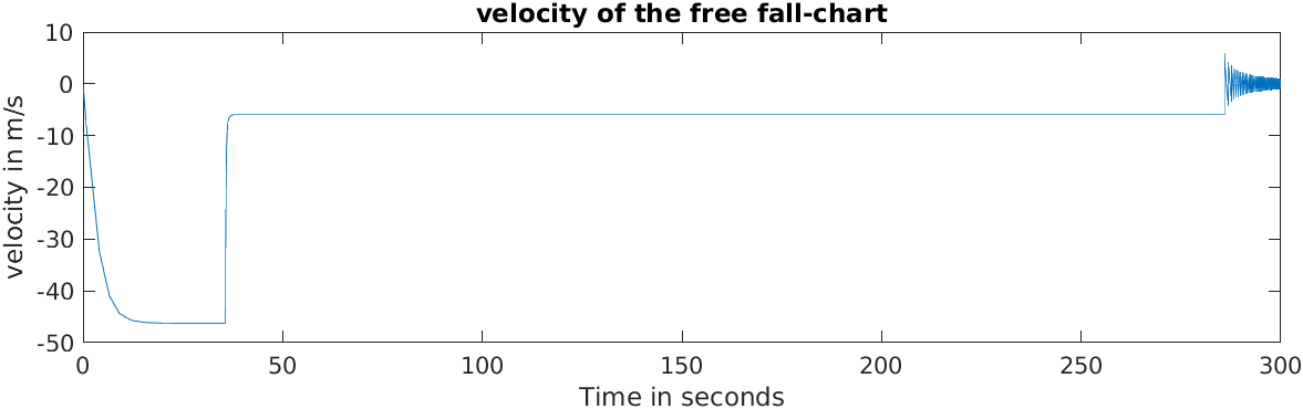
title('velocity of the free fall-chart');
subplot(3,1,2)
plot(out.simout.time,out.simout.signals.values(:,2));
xlabel('time in seconds');
ylabel('height in meter');
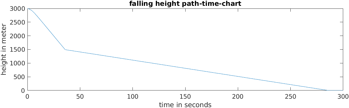
title('falling height path-time-chart');
subplot(3,1,3)
plot(out.simout.time,out.simout.signals.values(:,2));
xlabel('time in seconds');
ylabel('heigth in meter');
title('velocity-time chart');
ylim([0,25])
xlim([270,310]);
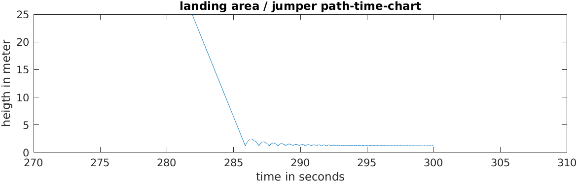
title('landing area / jumper path-time-chart')
%developed during a lecture / computer simulation of mechtronic systems
%evolved example from the book "Helmut Scherf- Modellbildung und %Simulation"
% Parameter Parachute Jumper
h_0 = 3000 ; % m height of the jump from plane
h_1 = 1500 ; % m height for open the parachute
h_test = 10 ;
h_SP = 1.2 ; % height of legs of the jumper touching the grond
A_S = 0.5 ; % m^2 bodysurface of the jumper
A_FS = 30 ; % m^2 surface ot the opened parachute
m_S = 85 ; % kg mass of the jumper
c_w_F = 1.3 ; % coefficient of drag of the air
rho = 1.2 ; % kg/m^3 air density assumed constant
g = 9.81 ; % m/s^2 gravity
SimTime = 300; %simulation time
k_O = 1/2*c_w_F*rho*A_FS %decay factor with opened parachute
k_L = 1/2*c_w_F*rho*A_S %decay factor of the jumper falling
k_F = 2*g*m_S/0.5; %jumper can carry twice of his
%mass devided with 0.5 Meter // a spring constant
k_D = 1/2*g*m_S/2;% proportionality damping factor of the velocity
h_SP = 1.2; % heigt of the point of mass of the jumper // stomach area
%PID-Controller parameter
k_p = -k_F; %P
k_d = -k_D; %D
k_i = -0.1*k_p; %I
%open simulation
%simfile = '$PATH'
%sim(simfile);
figure(3); %plot it
subplot(3,1,1)
plot(out.simout.time,out.simout.signals.values(:,1));
xlabel('Time in seconds');
ylabel('velocity in m/s');
title('velocity of the free fall-chart');
subplot(3,1,2)
plot(out.simout.time,out.simout.signals.values(:,2));
xlabel('time in seconds');
ylabel('height in meter');
title('falling height path-time-chart');
subplot(3,1,3)
plot(out.simout.time,out.simout.signals.values(:,2));
xlabel('time in seconds');
ylabel('heigth in meter');
title('velocity-time chart');
ylim([0,25])
xlim([270,310]);
title('landing area / jumper path-time-chart')
Simulation plots
In the first chart we see the jumper falling until the parachute opens and the velocity of the jumper stays at around 5 m/s. After about 280 seconds the jumper touches the ground and the velocity alternates for a while because of the impulses while tapping the ground until it stops. In the second chart we see that the parachute is opened at a height of 1500 meter from the ground. The chart 3 is limited to the point of time the jumper lands with a decaying movement.